SDAR-Algorithm

Run the SDAR-algorithm as standardized in "ASTM E3076-18". Will use numerous linear regressions (.lm.fit() from the stats-package) and can be painfully slow for test data with high resolution. See the article Speed Benchmarking the SDAR-algorithm for further information.

Usage

sdar(data, x, y, verbose = TRUE, plot = TRUE, ...)

Arguments

data: Data record to analyze. Labels of the data columns will be used as units.
x, y: <tidy-select> Columns with x and y within data.
verbose, plot: Give a summarizing report / show a plot of the final fit.
...: <dynamic-dots> Pass parameters to downstream functions: e.g. set verbose.all or plot.all to get additional diagnostic information during processing data.

Value

A list containing a data.frame with the results of the final fit, lists with the quality- and fit-metrics, and a list containing the crated plot-functions.

Note

The function can use parallel processing via the furrr-package. To use this feature, set up a plan other than the default sequential strategy beforehand.

References

Lucon, E. (2019). Use and validation of the slope determination by the analysis of residuals (SDAR) algorithm (NIST TN 2050; p. NIST TN 2050). National Institute of Standards and Technology. https://doi.org/10.6028/NIST.TN.2050

Standard Practice for Determination of the Slope in the Linear Region of a Test Record (ASTM E3076-18). (2018). https://doi.org/10.1520/E3076-18

Graham, S., & Adler, M. (2011). Determining the Slope and Quality of Fit for the Linear Part of a Test Record. Journal of Testing and Evaluation - J TEST EVAL, 39. https://doi.org/10.1520/JTE103038

Examples

# Synthesize a test record resembling EN AW-6060-T66
# Explicitly set names to "strain" and "stress",
# set effective number of bits in the x-data to 12
# to limit the number of data points.

Al_6060_T66 <- synthesize_test_data(
  slope = 69000,
  yield.y = 160,
  ultimate.y = 215,
  ultimate.x = 0.08,
  x.name = "strain",
  y.name = "stress",
  toe.start.y = 3, toe.end.y = 10,
  toe.start.slope = 13600,
  enob.x = 12
)


# use sdar() to analyze the synthetic test record
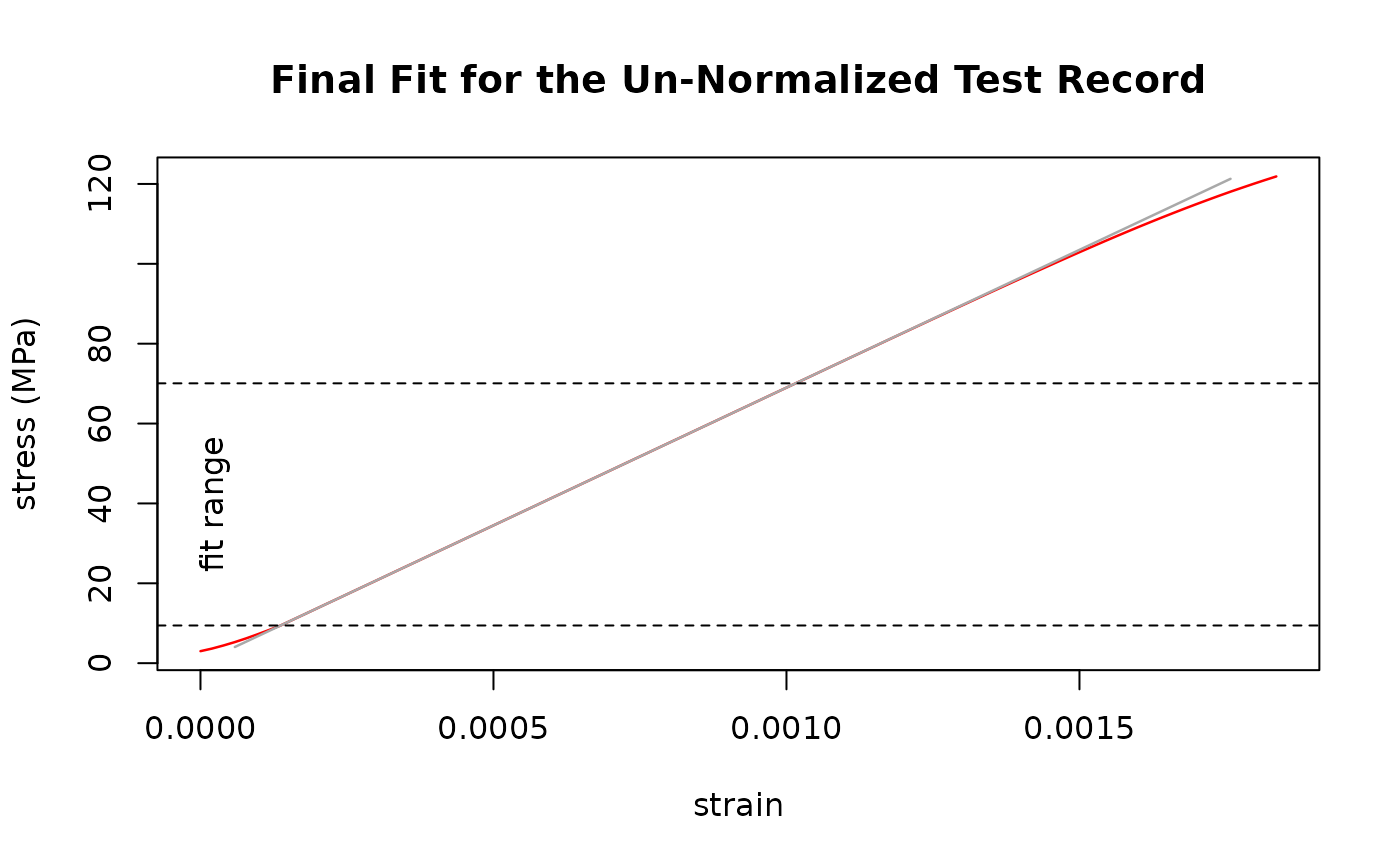
# will print a report and give a plot of the final fit
# \donttest{
result <- sdar(Al_6060_T66, strain, stress)
#> Determination of Slope in the Linear Region of a Test Record:
#> SDAR-algorithm
#>   Data Quality Metric: Digital Resolution
#>     x
#>       Relative x-Resolution:   0.333333333333333
#>       % at this resolution:    0
#>       % in zeroth bin:         100
#>       --> pass
#>     y
#>       Relative y-Resolution:   0.333333333333333
#>       % at this resolution:    10.752688172043
#>       % in zeroth bin:         82.7956989247312
#>       --> pass
#>   Data Quality Metric: Noise
#>     x
#>       Relative x-Noise:        9.44216060311802e-15
#>       --> pass
#>     y
#>       Relative y-Noise:        0.25059496508498
#>       --> pass
#>   Fit Quality Metric: Curvature
#>     1st Quartile
#>       Relative Residual Slope: 0.000341884560090671
#>       Number of Points:        12
#>       --> pass
#>     4th Quartile
#>       Relative Residual Slope: -0.00714862515119831
#>       Number of Points:        12
#>       --> pass
#>   Fit Quality Metric: Fit Range
#>       relative fit range:      0.784159272884657
#>       --> pass
#>   Un-normalized fit
#>       Final Slope:             68997.5639839654 MPa
#>       True Intercept:          0.00119126773051326 MPa
#>       y-Range:                 9.43511962890625 MPa - 70.074462890625 MPa

# }