Random Sub-Sampling Variant of the SDAR-Algorithm

Run a random sub-sampling modification of the SDAR algorithm as standardized in "ASTM E3076-18". As the original version uses numerous linear regressions (.lm.fit() from the stats-package), it can be painfully slow for test data with high resolution. The lazy variant of the algorithm will use several random sub-samples of the data to find an estimate for the fit-range within the data and thus can improve processing speed. See the article Speed Benchmarking the SDAR-algorithm for further information.

Usage

sdar_lazy(
  data,
  x,
  y,
  verbose = TRUE,
  plot = TRUE,
  n.fit = 5,
  cutoff_probability = 0.5,
  ...
)

Arguments

data: Data record to analyze. Labels of the data columns will be used as units.
x, y: <tidy-select> Columns with x and y within data.
verbose, plot: Give a summarizing report / show a plot of the final fit.
n.fit: Repetitions of drawing a random sub-sample from the data in the normalized and finding a fitting range to find an estimate for the final fitting range.
cutoff_probability: Cut-off probability for estimating optimum size of sub-sampled data range via logistic regression, which is predicting if sub-sampled data will pass the quality checks.
...: <dynamic-dots> Pass parameters to downstream functions: e.g. set verbose.all or plot.all to TRUE to get additional diagnostic information during processing data. Set enforce_subsampling to TRUE to run the random sub-sampling algorithm even though it might be slower than the standard SDAR-algorithm.

Value

A list containing a data.frame with the results of the final fit, lists with the quality- and fit-metrics, and a list containing the crated plot-functions.

Note

The function can use parallel processing via the furrr-package. To use this feature, set up a plan other than the default sequential strategy beforehand. Also, as random values are drawn, set a random seed beforehand to get reproducible results.

References

Lucon, E. (2019). Use and validation of the slope determination by the analysis of residuals (SDAR) algorithm (NIST TN 2050; p. NIST TN 2050). National Institute of Standards and Technology. https://doi.org/10.6028/NIST.TN.2050

Standard Practice for Determination of the Slope in the Linear Region of a Test Record (ASTM E3076-18). (2018). https://doi.org/10.1520/E3076-18

Graham, S., & Adler, M. (2011). Determining the Slope and Quality of Fit for the Linear Part of a Test Record. Journal of Testing and Evaluation - J TEST EVAL, 39. https://doi.org/10.1520/JTE103038

Examples

# Synthesize a test record resembling EN AW-6060-T66.
# Explicitly set names to "strain" and "stress".

Al_6060_T66 <- synthesize_test_data(
  slope = 69000,
  yield.y = 160,
  ultimate.y = 215,
  ultimate.x = 0.08,
  x.name = "strain",
  y.name = "stress",
  toe.start.y = 3, toe.end.y = 10,
  toe.start.slope = 13600
)


# use sdar_lazy() to analyze the (noise-free) synthetic test record
# will print a report and give a plot of the final fit
# \donttest{
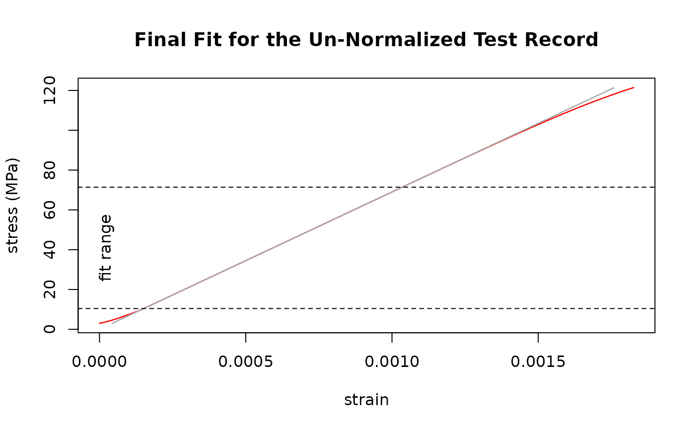
result <- sdar_lazy(Al_6060_T66, strain, stress)
#> Determination of Slope in the Linear Region of a Test Record:
#> Random sub-sampling modification of the SDAR-algorithm
#>   Random sub-sampling information:
#>       121 points of 375 points in the normalized range were used.
#>       0 % of the sub-samples passed the data quality checks.
#>       100 % of the sub-samples passed the fit quality checks.
#>       0 % of the sub-samples passed all quality checks.
#>   
#>   Data Quality Metric: Digital Resolution
#>     x
#>       Relative x-Resolution:   0.333333333333333
#>       % at this resolution:    0
#>       % in zeroth bin:         100
#>       --> pass
#>     y
#>       Relative y-Resolution:   0.333333333333333
#>       % at this resolution:    0.804289544235925
#>       % in zeroth bin:         99.1957104557641
#>       --> pass
#>   Data Quality Metric: Noise
#>     x
#>       Relative x-Noise:        1.14246654063749e-14
#>       --> pass
#>     y
#>       Relative y-Noise:        0.0619676935307803
#>       --> pass
#>   Fit Quality Metric: Curvature
#>     1st Quartile
#>       Relative Residual Slope: 0.00086452510296137
#>       Number of Points:        46
#>       --> pass
#>     4th Quartile
#>       Relative Residual Slope: -0.00711062691360424
#>       Number of Points:        46
#>       --> pass
#>   Fit Quality Metric: Fit Range
#>       relative fit range:      0.777012483857081
#>       --> pass
#>   Un-normalized fit
#>       Final Slope:             68997.0676230752 MPa
#>       True Intercept:          0.00127687293251233 MPa
#>       y-Range:                 10.445556640625 MPa - 71.4129638671875 MPa

# }