Random sub-sampling variant of the SDAR-algorithm

Run a random sub-sampling modification of the SDAR algorithm as originally standardized in ASTM E3076-18. As the original version uses numerous linear regressions (.lm.fit() from the stats-package), it can be painfully slow for test data with high resolution. The lazy variant of the algorithm will use several random sub-samples of the data to find the best estimate for the fit-range within the data and thus can speed up calculations. See the article Speed Benchmarking the SDAR-algorithm for further information. Additionally, the test data can be de-noised using Variational Mode Decomposition in case initial data quality checks have failed (highly experimental).

Usage

sdar.lazy(
  data,
  x,
  y,
  verbose = TRUE,
  plot = TRUE,
  plotFun = FALSE,
  n.fit = 5,
  cutoff_probability = 0.5,
  ...
)

Arguments

data: Data record to analyze. Labels of the data columns will be used as units.
x, y: <tidy-select> Columns with x and y within data.
verbose, plot: Give a summarizing report / show a plot of the final fit.
plotFun: Set to TRUE to get a plot-function for the final fit with the results for later use.
n.fit: Repetitions of random sub-sampling and fitting.
cutoff_probability: Cut-off probability for estimating optimum size of sub-sampled data range via logistic regression.
...: <dynamic-dots> Pass parameters to downstream functions: set verbose.all, plot.all and plotFun.all to TRUE to get additional diagnostic information during processing data. Set enforce_subsampling to TRUE to run the random sub-sampling algorithm even though it might be slower than the standard SDAR-algorithm.

Value

A list containing a data.frame with the results of the final fit, lists with the quality- and fit-metrics, and a list containing the crated plot-function(s) (if plotFun = TRUE or, for all diagnostic plots plotFun.all = TRUE).

Note

The function can use parallel processing via the furrr-package. To use this feature, set up a plan other than the default sequential strategy beforehand. Also, as random values are drawn, set a random seed beforehand to get reproducible results.

References

Lucon, E. (2019). Use and validation of the slope determination by the analysis of residuals (SDAR) algorithm (NIST TN 2050; p. NIST TN 2050). National Institute of Standards and Technology. https://doi.org/10.6028/NIST.TN.2050

Standard Practice for Determination of the Slope in the Linear Region of a Test Record (ASTM E3076-18). (2018). https://doi.org/10.1520/E3076-18

Graham, S., & Adler, M. (2011). Determining the Slope and Quality of Fit for the Linear Part of a Test Record. Journal of Testing and Evaluation - J TEST EVAL, 39. https://doi.org/10.1520/JTE103038

Dragomiretskiy, K., & Zosso, D. (2014). Variational Mode Decomposition. IEEE Transactions on Signal Processing, 62(3), 531–544. https://doi.org/10.1109/TSP.2013.2288675

Examples

# Synthesize a test record resembling Al 6060 T66
# (Values according to Metallic Material Properties
# Development and Standardization (MMPDS) Handbook).
# Explicitly set names to "strain" and "stress".

Al_6060_T66 <- synthesize_test_data(
  slope = 68000,
  yield.y = 160,
  ultimate.y = 215,
  ultimate.x = 0.091,
  x.name = "strain",
  y.name = "stress",
  toe.start.y = 3, toe.end.y = 10,
  toe.start.slope = 13600
)


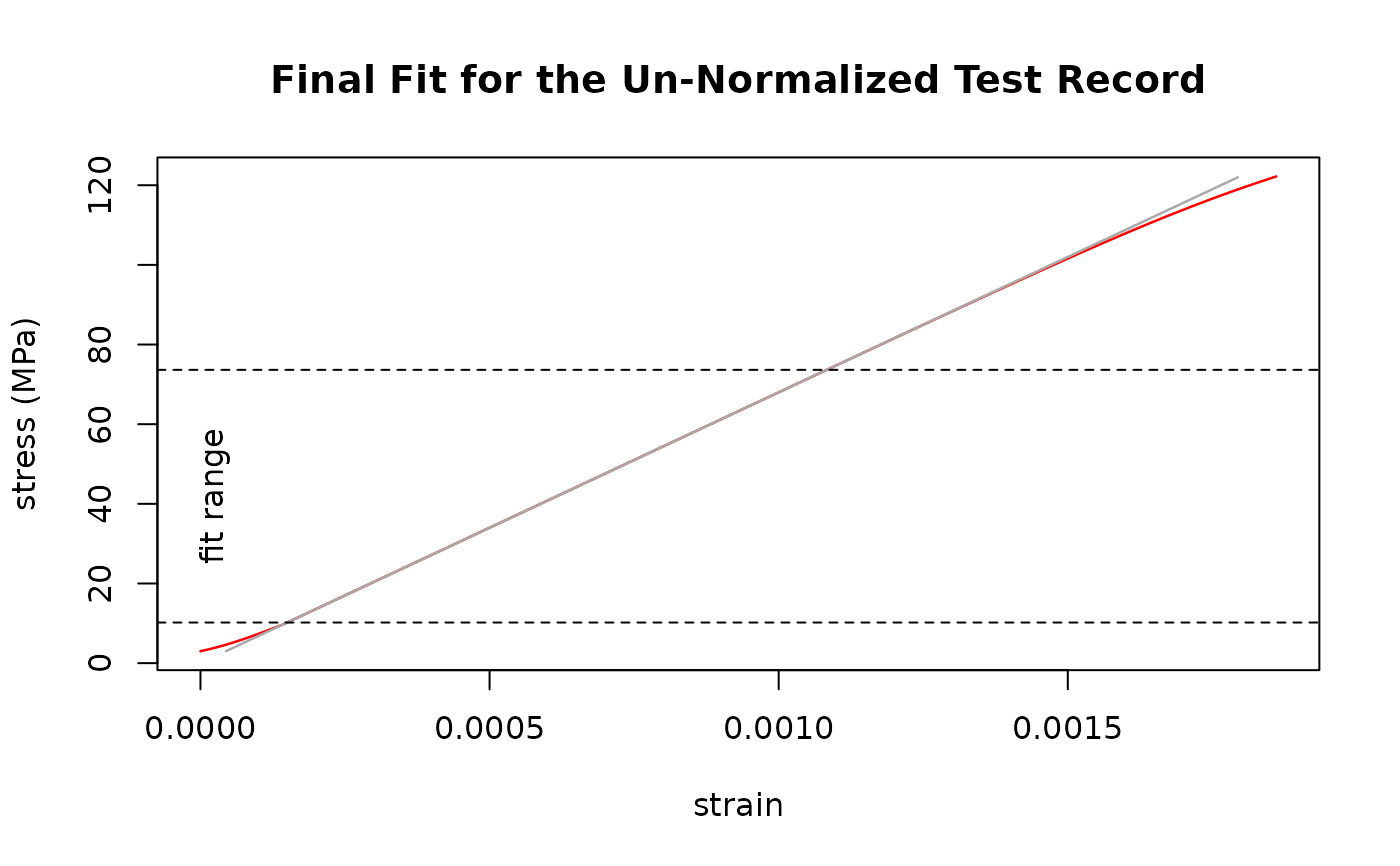
# use sdar.lazy() to analyze the (noise-free) synthetic test record
# will print a report and give a plot of the final fit
# \donttest{
result <- sdar.lazy(Al_6060_T66, strain, stress)
#> Determination of Slope in the Linear Region of a Test Record:
#> Random sub-sampling modification of the SDAR-algorithm
#>   Random sub-sampling information:
#>       120 points of 336 points in the normalized range were used.
#>       0 % of sub-sampled normalized ranges passed the data quality checks.
#>       100 % of linear regressions passed the fit quality checks.
#>       0 % of linear regressions passed all quality checks.
#>   
#>   Data Quality Metric: Digital Resolution
#>     x
#>       Relative x-Resolution:   0.333333333333333
#>       % at this resolution:    0
#>       % in zeroth bin:         100
#>       --> pass
#>     y
#>       Relative y-Resolution:   0.666666666666667
#>       % at this resolution:    0.29940119760479
#>       % in zeroth bin:         99.7005988023952
#>       --> pass
#>   Data Quality Metric: Noise
#>     x
#>       Relative x-Noise:        8.92753747230055e-15
#>       --> pass
#>     y
#>       Relative y-Noise:        0.067704464397069
#>       --> pass
#>   Fit Quality Metric: Curvature
#>     1st Quartile
#>       Relative Residual Slope: 0.00111396508829732
#>       Number of Points:        43
#>       --> pass
#>     4th Quartile
#>       Relative Residual Slope: -0.00587104306414906
#>       Number of Points:        42
#>       --> pass
#>   Fit Quality Metric: Fit Range
#>       relative fit range:      0.751520165460186
#>       --> pass
#>   Un-normalized fit
#>       Final Slope:             67997.1403217637 MPa
#>       True Intercept:          0.00128197955692277 MPa
#>       y-Range:                 10.1962280273438 MPa - 73.643798828125 MPa

# }